Interesting Problems in Decision Theory
Today's post is all about decision theory, the art (or science) of making real world decisions based on statistical models. Decision theory is one of my favorite topics in statistics, but is often neglected in the classroom, and many students find themselves woefully ill equipped to tackle problems involving decision theory.
I thought that it would be fun to explore a few fun problems in decision theory. We'll start with a very simple problem (that is covered in many introductory statistics classes), then move on to a problem that is closer to what a statistician working in the real world might encounter, and finally end with an advanced (and perplexing) problem. If you enjoy this taste of decision theory, I recommend diving into Statistical Decision Theory and Bayesian Analysis by James Berger for a full treatment of the field.
Overview:
- The Monty Hall Problem
- Issues in Marketing
- St. Petersburg Paradox
The Monty Hall Problem
Yes yes ... collective sigh from anyone that has taken a college level stats course. The Monty Hall problem is SO over done. Well, feel free to skip this first section if you are already too familiar with the Monty Hall problem. I, personally, love the Monty Hall problem. It's often the first example students encounter of using statistics to make a decision that is counter to their naive intuition. It's almost a rite of passage for aspiring statisticians (perhaps I'm romanticising a simple math exercise to excess).
The Problem
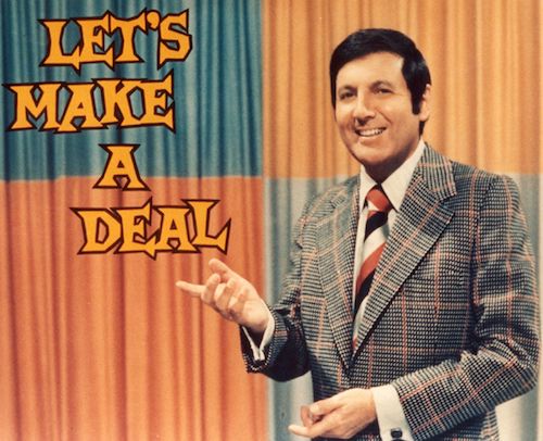
So, what's the problem? Imagine you are on a game show called "Let's Make a Deal" (hosted by the famous Monty Hall).
The game is very simple. At first you are shown three doors. Behind one door is a brand new car! Behind the other two doors are goats (one goat for each door, not a herd of goats). You are asked to select a single door.
Once you have selected a door, the game show host (Monty Hall) opens one of the remaining doors to reveal a goat. There are now two doors left unopened (one that you selected and one that you did not).
You are asked to select one of the remaining doors. Do you stay with your initial choice or do you switch choices?
Many stats novices say that it doesn't matter. There are two doors left so there is a 50/50 chance you pick the correct door. WRONG! It turns out that the probability is not split 50/50 between the remaining two doors.
Decision Theoretic Solution
It seems that intuition has failed us. Let's use statistics to inform our choice (aka decision theory). At the beginning of the game we are asked to select one of three doors. Is there an optimal action/policy/choice? (action, policy, and choice are often used interchangeably in decision theory and reinforcement learning) Let's assume that the car is placed perfectly randomly behind one of the doors. Under this assumption there is not best choice of door. You should just pick randomly.
So far the decision theoretic strategy and intuition are perfectly aligned.
Let's say that you randomly picked door One. The game show host now walks over and opens door Three. This leaves doors One and Two unopened. You are asked to pick one of the remaining doors. Should you stick with your first pick or change your pick?
Well, at the beginning there was $\frac{1}{3}$ chance that the car was behind each of the doors. You chose door One, so there is a $\frac{2}{3}$ chance that the car is behind either door Two or door Three. The odds are not in your favor. However, Monty Hall helps you out! He opens one of the doors that you did not pick. Now we know that Monty Hall will never open the door with the car behind it. There is a 0% chance that he opens the door with the car.
In our example we said that Monty Hall opens door Three. Before he opened Three there was a $\frac{2}{3}$ chance that the car was behind either Two or Three. When he opened Three we immediately realize that there is a $\frac{0}{3}$ chance that the car is behind Three! That means that there must be a $\frac{2}{3}$ chance that the car is behind door Two.
WAIT! That's completely different from the common intuition novices have that after the door is opened there is a 50/50 chance that the car is behind either of the two remaining doors. This is the trick of the Let's Make a Deal game show.
If you stick with your original door you have a $\frac{1}{3}$ chance of winning the car (the same odds as before one of the doors was revealed). Because you know that Monty Hall will never open the door with the car behind it, we are able to deduce that the unopened door that you did not originally pick has a $\frac{2}{3}$ chance of having the car behind it. If you switch you choice the odds are now in your favor!
The decision theoretic optimal policy is to always switch your choice after Monty Hall reveals on of the unpicked doors.
A More Formal Treatment
The statistical analysis above was a bit hand wavy. Let's actually do some calculations to confirm our results. I'll be using Bayesian methods. Frequentist methods yield the exact same answer.
Let's Assume the we initially choose door One. Monty Hall then opens door Three. What are the probabilities that the car is behind doors One or Two.
$$ P(Car=1|Opened=3) = \cfrac{P(Opened=3|Car=1)P(Car=1)}{P(Opened=3)} = \cfrac{\frac{1}{2} * \frac{1}{3}}{\frac{1}{2}} = \frac{1}{3} $$$$ P(Car=2|Opened=3) = \cfrac{P(Opened=3|Car=2)P(Car=2)}{P(Opened=3)} = \cfrac{1 * \frac{1}{3}}{\frac{1}{2}} = \frac{1}{3} = \frac{2}{3} $$Confirming Our Analysis
Now some of you might still be skeptical of our statistical treatment. Let's run some Monte Carlo simulations of the Monte Hall problem and see if the probabilities we came up with above actually hold true.
import numpy as np
import numpy.random as rand
import matplotlib.pyplot as plt
def monty_hall_simulations():

    # possible doors to choose from
    doors = [1, 2, 3]

    # pick the contestant's initial choice and
    # the winning door randomly
    initial_door_choice = rand.randint(1, 4, 1)
    winning_door = rand.randint(1, 4, 1)

    if initial_door_choice == winning_door:

        # if the contestant's initial choice is the
        # winning car then Monty Hall randomly chooses
        # one of the remaining doors to open
        doors.remove(initial_door_choice)
        open_door = rand.choice(doors)
        switch_door = doors.remove(open_door)

    else:

        # if the contestant does not initially pick
        # correctly then Monty Hall must open the
        # unselected door with the goat so as not
        # to reveal the car
        doors.remove(initial_door_choice)
        doors.remove(winning_door)
        open_door = doors
        switch_door = winning_door

    # a simulated win is a 1 and a
    # simualted loss is a 0
    if switch_door == winning_door:
        switch = 1
        dont_switch = 0
    else:
        switch = 0
        dont_switch = 1

    return [switch, dont_switch]
num_simulations = 10000

simulations = np.asarray([
    monty_hall_simulations() for _ in range(num_simulations)
])

switch_victories = 100.0 * simulations[:, 0].sum() / num_simulations
dont_switch_victories = 100.0 * simulations[:, 1].sum() / num_simulations

print("Switching Resulted in Victory {}% of Games".format(switch_victories))
print("Not Switching Resulted in Victory {}% of Games".format(dont_switch_victories))
As you can see, the simulations confirm our analysis! Switching is the better strategy.
Issues in Marketing
We just went through a very simple example of using decision theory to guide our actions in a game show. The rewards were very clear (frankly, they were black and white) and the probabilities were simple. In this example we'll try to make things a bit more complicated to get a feel for how we might apply decision theory to an actual business problem many statisticians face in the real world.
Let's imagine that we are part of the corporate strategy team for a major toy company. Our research and development (R&D) department has come up with three new toys. Our CEO tells us to decide on a single product/toy to market. Which toy do we market?
Well, luckily for us, the business analysts in marketing have developed models to try to predict what profit we might expect from each potential product marketing strategy. These models are based on past tests that the marketing team has run as well as decades of expert knowledge. Marketing realizes that the forecasting models are not perfect and so design the models to output a range of predictions (perhaps using Bayesian methods!). For simplicity's sake, we assume the model just outputs two predictions: favorable projection and unfavorable projection (in a more realistic example the models might output a distribution, i.e. a Gaussian posterior over profits).
Below is a table showing the toys R&D developed as well as the profit projections from the Marketing team.
| Product | Favorable Projection Profit | Unfavorable Projection Profit |
|---|---|---|
| Toy A | \$5000 | -\$1000 |
| Toy B | \$10000 | -\$3000 |
| Toy C | \$3000 | -\$500 |
We also show a table with estimated probabilities for each of Marketing's projected scenarios.
| Product | Favorable Projection Profit | Unfavorable Projection Profit |
|---|---|---|
| Toy A | 80% | 20% |
| Toy B | 60\% | 40% |
| Toy C | 50% | 50% |
What do we do with this information? Well, a rational person might say that they want to make the action that maximizes the expected return. How do we calculate the expected return? That's actually very simple! The expected return for a particular action is the sum of each possible return times the probability of that return.
For example, the expected return if we choose to market Toy A is:
$$ E[Return] = \sum_i^N Reward_i * Pr_i = 5000 * 0.8 + -1000 * 0.2 = 4000 - 200 = 3800 $$The table below shows the results of our calculations.
| Product Choice | Favorable Projection | Unfavorable Projection | Expected Payoff |
|---|---|---|---|
| Toy A | \$5000 * 80\% = \\$4000 | -\$1000 * 20\% = -\\$200 | \$3800 |
| Toy B | \$10000 * 60% = \\$6000 | -\$3000 * 40% = -\\$1200 | \$4800 |
| Toy C | \$2000 * 50\% = \\$1500 | \$500 * 50\% = -\\$250 | \$1250 |
The expected maximum payoff is to market Toy B. That should probably be our recommendation to the CEO. While the models most companies use for valuations are much more complicated than the example above, the overall methodology for making decisions is the same. This comprised much of the work I've done in the finance industry over the past 3-4 years.
The St. Petersburg Paradox
Okay, now for the super fun stuff! One of my friends (Mack Sweeney) posed this fun thought experiment to me at work last week. The St. Petersburg paradox is an interesting conundrum in decision theory first mentioned by Nicolas Bernoulli in 1713.
Let's propose a game! At the start of the game the player pays an entry fee. The entry fee is the only cost for the player for the entire game (i.g. the player will lose no more money than what he or she pays to play). The upside, however, is variable.
The game is played by flipping a coin. When the coin comes up heads the game is stopped. For every flip of the coin the payout is doubled starting at $2. If the first flip is heads then the payout is 2 dollars. If the third flip ends up as heads then the payout is 2 x 2 x 2 = 8. The coin flips are perfectly random (the coin is fair) and independent of each other.
How much would you be willing to pay as the entry fee for the game?
Well, in the last example we used the expected payout to make our decision. We could do the same here and say, "I'd be willing to pay up to the expected payout of the game to play". This seems reasonable on the face of it. If we paid the expected payout then we would, over the long term, break even playing the game. If we pay less than the expected return then we will, over the long term, be net positive playing the game.
So what is the expected payout?
$$ E[Reward] = \sum_i^N Return_i * Pr_i = \sum_0^\infty Return_i * Pr_i = 2 * \frac{1}{2} + 4 * \frac{1}{4} + 8 * \frac{1}{8} + ... = 1 + 1 + 1 + 1 + ... = \infty $$Uh oh, the expected payout is infinite? (This is why even mathematician should know his or her limits) Would you be willing to pay up to everything you own to play this game? Most people say no. This is the paradox. Decision theory gives us an answer that simply doesn't reconcile with our intuition.
How can we explain this paradox? Well, there are a number of very intelligent people that have tried to explain this paradox in terms of math and psychology (see HERE). Below I'll give some of my thoughts on the matter.
Explanation One: Near Zero IS Zero
My first attempt is going to be a hand wavy nod in the direction of psychology (you've been warned). When humans make decisions they don't deal in actual percentages. For example, if you were trying to judge if you could make a jump across a canyon, you would think "I could probably (or probably not) make that jump". At no point did you assign an actual probability to the outcome of the jump (like 22% for instance). This means that high probabilities of success (like 99.999999%) essentially become 100% and low probabilities of success (like 0.00000001%) essentially become 0%.
This means that the long tail of probabilities that lead to the infinite expected reward for the coin flipping game are all rounded to zero by "human intuition". They are so unlikely that they are essentially impossible. This might help explain why intuition balks at the idea of paying a large sum of money for playing. Many people might not be willing to play the game for any meaningful amount of money at all!
Explanation Two: Risk Adversity
Even if explanation one is correct, we should still be able to come up with an amount we would be willing to pay to play the game. Let's try to actually find the amount we would be willing to pay.
First let's ask the question, "what is the probability of not seeing a single heads in 15 consecutive coin flips?" It's a simple question. The answer is $\frac{1}{2}^{15}$. THis means that there is a 0.0031% chance of seeing not a single heads in 15 consecutive coin flips.
I think many rational humans would be willing to say that 0.0031% is essentially 0%. Given this we can say that any result with a probability <= 0.0031% is essentially impossible. So what would we be willing to pay?
$$ E[Reward] = 2 * \frac{1}{2} + 4 * \frac{1}{4} + ... 16384 * \frac{1}{16384} = 1 + 1 + 1 ... + 1 = \$14 $$That doesn't actually seems like such a horrible result. I think plenty of people would pay $14 to play this game.
Explanation Three: Catastrophic Failure
Explanations one and two (which are basically a single explanation anyway) depend on a foible in human psychology. My friend Mack actually pointed this out (to my chagrin) and made a small tweak to the problem (one reason I hate hypotheticals). What if the player was not human? What if the player was a perfectly rational robot?
Would the robot be willing to pay everything it owned to play the game (assuming it was a rational but greedy robot)?
My answer is No. Why? Because we live in a volatile and finite universe! Sorry to wax philosophic, but this really is my answer. Let's imagine that the robot will turn off if it can't pay it's electric bill (equivalent to dying for a human and undesirable for the robot). If the robot is willing to pay everything it owns to play the game then it risks not being able to pay the electric bill for the month ... which is equivalent to death!
Even if the expected gain is infinite in the long run, there is a tangible risk of catastrophic failure in the near present. In fact, there is a 50\% chance of a $2 return playing the game. That means that there is at least a 50% chance that the robot will not be able to pay its (presumably high) electric bill that month if it pays everything it has to play.
The price the robot would be willing to play would be some function of the probability that it could not pay it's electric bill if it played the game. For example, if the robot had a monthly income of \$1000 and a monthly electric bill of \\$300, then the robot might be willing to pay \$702 to play the game once a month (remember that there is a guaranteed $2 minimum payout). This is the most that the robot could pay and still avoid catastrophic failure.
I keep using the term "catastrophic failure". What do I mean by that? I mean a failure that out weighs any possible return (such as death).
Practical Implications of Explanation Three
This has interesting implications for a number of problems in decision theory. For example, imagine that a company that has to make a choice between two products. The first product has a revenue stream with an expected monthly return of \$400. The second product has an expected monthly revenue stream of \\$1000. Which would you choose?
Up until now everyone in the room would pick the second product! But the St. Petersburg paradox might have introduced some doubt in your mind.
What if I said that the first revenue stream is very stable. The minimum revenue from the first revenue stream is \$100. The second revenue stream is very volatile. You can often expect (indeed it is very likely) that would will make \\$0 in a month. Not only that, but you have fixed monthly operational expenses of \$50 month that are required to keep your company open.
The risk adverse side of you brain is probably squealing by this point. Despite the high expected return of the second revenue stream there is some tangible chance that you won't be able to make operating expenses at some point in the future. That would mean that revenue stream might destroy the entire company (a catastrophic failure)!
The expected (or long term) return just doesn't seem to be the only piece of information required to make real world decisions. THis is one reason why decision theory can be so complicated.
Final Thoughts
I hope you enjoyed today's blog post! A lot of the concepts covered here are simplified versions of what big companies do every day. Making decisions with millions of dollars is often a function of risk and reward and the primary concerns of decision theory.